Page 87 - 《橡塑技术与装备》英文版2026年1月

TEST AND ANALYSIS

2.5 The influence of temperature on degradation energy Ea can be determined by the slope of lnk versus 1/T.
rate （ TE） f = (T × E b ) before aging After aging, the stress-strain properties of EPDM
b
)
E
(T ×
There are precedents for the application of the Arrhenius vulcanized rubber decrease, and the Arrhenius relationship can
b
b
after aging
relationship in elastomers and plastic materials. According to be used to predict the changes at different temperatures and
 1/ (TE ) − 1/ a  = k t '
'


the Arrhenius equation, as shown in equation (3): durations. The activation energy (E a ) value is determined by
f
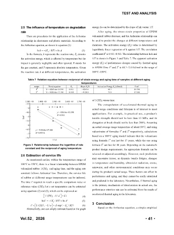
ln k = − (E a / RT + ln A (3) logarithmic linear regression of k against 1/T. The correlation
）
2
In the formula, k represents the reaction rate, E a denotes coefficient R is 0.911~0.911. The relationship between ln k and
 1/ (TE ) − 1/ a  = k t '
'


the activation energy, which is affected by temperature but the 1/T is shown in Figure 3 and Table 7. The apparent activation
f
impact is generally negligible and often ignored. R stands for energy (E a ) of performance changes caused by thermal aging
E
/ RT +
ln '
'
A
'
ln k = −（
）
a
#
#
the gas constant, and T represents absolute temperature. Given in EPDM films 1 and 2 is 68.7~75.8 kJ/mol in the range of
f −
' t =

'
E
exp −
'
A
'
1/ a ÷
1/ (TE）
（
/ RT）
the reaction rate k at different temperatures, the activation 100℃~150℃.


a
Table 7 Relation equation between reciprocal of strain energy and aging time of samples at different aging
temperatures
recipe Trend equation R 2 Slope-E a /R Activation Energy E a (kJ/mol) LnA’
1 # Y=-8263.6x+15.398 0.911 -8263.6 68.7 15.398
2 # Y=-9120.8x+17.188 0.958 -9120.8 75.8 17.188
of 1/(TE) f versus time.
The extrapolation of accelerated thermal aging to
actual usage conditions and lifespan is of interest to most
applications. For example, in practical use, a product's
tensile strength should not be less than 13 MPa, and its
elongation at break should not be less than 200%. Assuming
an actual average usage temperature of about 50°C, and using
vulcanizates of formulas 1 and 2 respectively, calculations
#
#
based on a 100°C aging model indicate that the vulcanizate
#
using formula 1 can last for 17 years, while the one using
Figure 3 Relationship between the logarithm of rate formula 2 can last for 44 years. Depending on the customer's
#
constant and the reciprocal of aging temperature product design requirements, the appropriate formula can be
2.6 Estimation of service life selected or adjusted accordingly. However, such predictions
As mentioned earlier, within the temperature range of may encounter issues, as dynamic tensile fatigue, changes
100°C to 150°C, there is a linear relationship between EPDM in temperature and humidity, ultraviolet radiation, ozone,
E
(T ×
) before aging
b
b
=
(T ×
E
（
vulcanized rubber 1/(TE) f and aging time, and the aging rate rainwater, and other environmental conditions may occur
TE） f
（ (T
) before aging
=
b
TE） f )E×
b
(T ×
E
b
) before aging
b
after aging
)
b
=
E
b
TE） f (T ×
（
constant follows Arrhenius' law. Therefore, the service life during the product's actual usage. These factors can affect its
E
)
b
after aging
b
(T ×
after aging
b
b
'
of rubber at different usage temperatures can be inferred. performance and aging, and they cannot be easily simulated

'
1/ a  =
k t
1/ (TE
) −


'
'

f
1/ a  =
) −
k t
1/ (TE

' 
'

1/ a  =
f
The time t' required to reach a specific comparison value or and predicted in the laboratory. Nevertheless, if thermal aging
k t
1/ (TE
) −


f
ln k = − (E / RT + ln A is the primary mechanism of deterioration in actual use, the
）
reference value ((TE) f f at a set temperature can be estimated
a
ln k = −
ln A
(E
/ RT +
）
ln A
ln k = −
/ RT +
(E
a
）
a
using equations (2) and (5), which can be expressed as: performance retention rate can be estimated from the results of
'
'

k t
1/ a  =
1/ (TE
) −


f
'

'
k t
) −
1/ a  =
1/ (TE
' 

  1/ (TE f ) − 1/ a  = k t ' (4) accelerated thermal aging in the laboratory.

f
'
A
）
ln k = −（ E a ' / RT + ln '
A
'
）
ln k = −（ E a ' / RT + ln ' (5)
'
A
ln k = −（ E a ' / RT + ln ' 3 Conclusion
）
'
't =   1/ (TE） 1/ a ÷ ' A ' exp − E ' ' a / RT） (6)
f −
（

E
1/ a ÷
f −
'

' t =
exp −
A
（
1/ (TE）
/ RT）


Alternatively, one can simply estimate based on the graph Based on the Arrhenius equation, a simple empirical
a

'
exp −
f −
1/ a ÷
' t =
A
'
E
'
/ RT）
1/ (TE）
（


a
Vol.52，2026 ·41·